Learning to Learn

Paper

arxiv.org/abs/2005.12320

Code

github.com/wvangansbeke/Unsupervised-Classification

Introduction

본 논문은 기존 unsupervised clustering 논문들과 다르게 two-step 형태의 approach를 사용했다는 것이 특징이다.

SCAN (Semantic Clustering by Adopting Nearest neighbors)의 과정은 다음과 같다.

- 첫번째는 기존의 Deep cluster가 represetation learning을 통한 classifier output을 통한 clustering 때문에 cluster degeneracy를 발생시키는 문제점을 대비해서 nearest neighbors를 이용해 clustering을 진행한다.

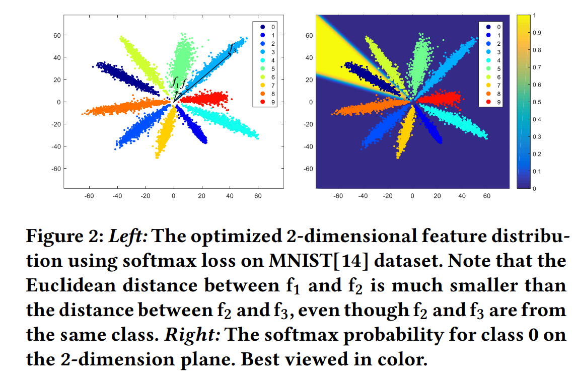
nearest neighbor도 same semantic class에 속하기 때문에 이것이 가능하다. (Fig 2)

- 두번째는 nearest neighbor들을 learning의 prior로 활용한다는 점이다. 이는 기존의 방법이 특정 sample과 그 sample에 하나의 augmentation을 적용한 sample을 가깝게 embedding 되도록 학습하는 것에 비해 nearest neighbor들을 가깝게 embedding 시킨다는 차이점이 있다.

Method

- 기존의 방법은 CNN의 prediction을 이용해 k-means clustering을 형성하고, k-means clustering을 통해 형성된 label을 통해 다시 CNN의 학습을 진행하는 것을 반복한다. 그러나 k-means의 초기 label은 네트워크가 학습이 덜 진행된 상태에서 결정되는 부분이기 때문에 high-level information을 추출한 상태가 아니게 되고 최종 목표인 semantic clustering에 오히려 방해가 되게 된다.

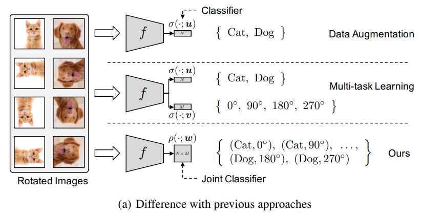
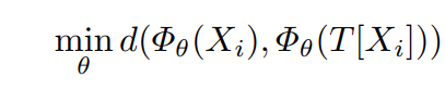
- 이를 해결하기 위해 representation-learning (self-supervised learning)을 활용한다. 기존의 self-supervised learning의 경우 특정 image에 transformation을 적용하고 각각에 대해 다른 label을 적용하여 다른곳에 embedding 되도록 한다. 그러나 이러한 방식은 유사한 이미지가 비슷한 곳에 위치되어야 하는 semantic clustering에 맞지 않기 때문에 다음과 같이 transformation을 적용한 것과 같은 곳에 위치하도록 loss function을 구성한다. (contrastive learning 참고) 

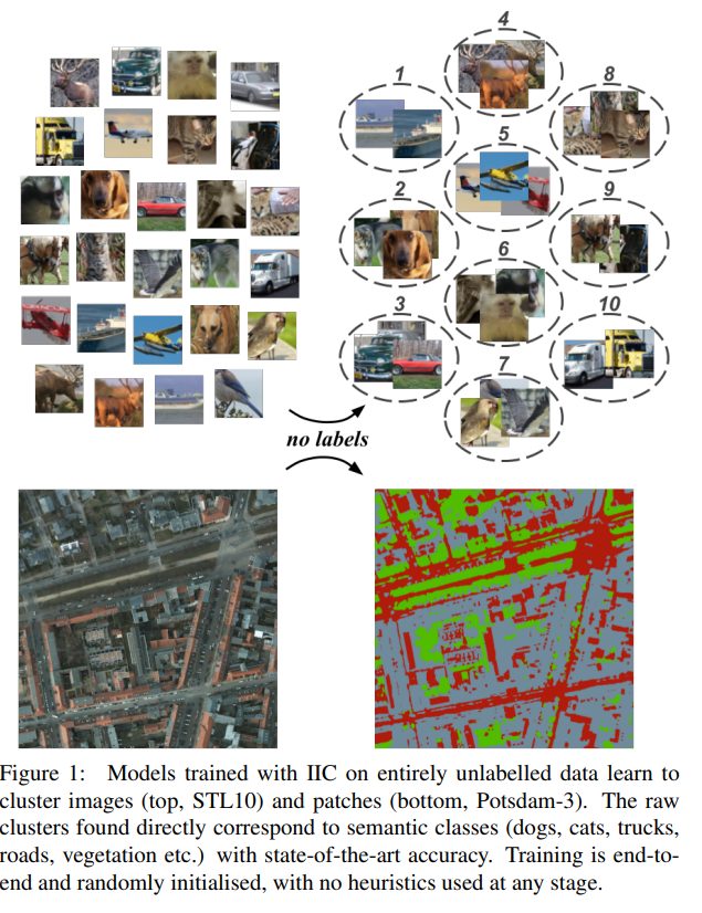
- 이와 같은 방법으로 유사한 class가 가깝게 위치하는 경향을 띄는 것을 실험으로 증명하였다. (Fig 1,2)

- 이러한 것이 가능한 이유는 다음과 같다. 첫번째는 모델 Φ_θ가 loss function에 의해서 특정 information을 추출하도록 유도된다. 두번째는 모델 Φ_θ가 추출하는 feature의 크기는 한정되어 있기 때문에 필요없는 information은 버리고, 필요한 high-level information만 추출한다. 

- 이러한 motivation으로 먼저 SimCLR이나 Moco와 같은 self-supervised learning을 이용해 feature를 학습하고 이 feature를 이용해 clustering을 진행한다. 그러나 단순히 이러한 방식으로는 cluster degeneracy를 막을 수 없다.

-때문에 본 논문에서는 nearest neighbor를 이용한다.

-먼저 self-supervised learning을 이용해 feature space를 형성한다. sample X_i에 대해서 K-nearest neighbor를 찾고 이를 N_X_i로 정의한다. 이때, N_X_i가 X_i랑 같은 label로 형성되는 것이 중요한 데, fig 2를 보면 같은 label로 형성되는 비율이 나와 있다. 결과적으로 유의미하게 같은 label로 형성된다고 판단되기에 저자는 k-nearest neighbor를 semantic clustering의 prior로 활용한다.

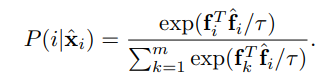
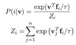
-위의 X_i와 N_X_i를 이용해 classification을 수행하는 새로운 모델 Φ_η을 학습한다. 이때 Φ_η는 맨 마지막단은 softmax function으로 구성되어 있으며,Φ_η(X_i)는 Φ_η 함수의 softmax output을 의미하며, Φ^c_η(X_i)는 X_i가 cluster c에 속하는 확률값만을 따로 추출한 것이다. 

- 첫번째 식은 X의 Φ_η 모델에 대한 softmax output과  X의 nearest neighbor에 대한 softmax output을 dot product한 결과이다. 이때, dot product가 최대가 되는 경우는 두개의 prediction이 one-hot label로 같게 되는 경우이다. 

(그렇게 해서 값이 1이 나오면 log (1)이 되어 loss는 0이 된다.

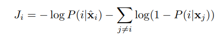
- 그러나 첫번째 식만 있는 경우, 모든 sample을 하나의 cluster로 prediction하는 cluster degeneracy가 발생하게 되고 때문에, 두번째 식 entropy식을 이용해 하나의 cluster로 모두 assign되는 현상을 막는다.

- entropy식의 마이너스를 loss function으로 활용함으로 sample들이 다양한 cluster에 assign되도록 만들어준다.

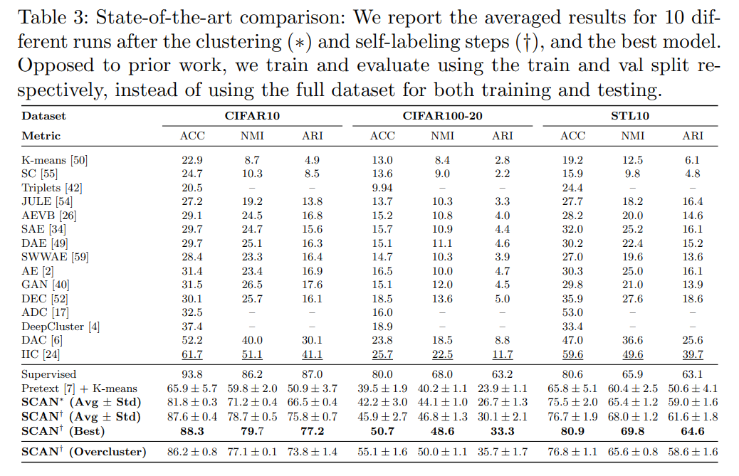
-이때, cluster 수는 실제로는 모르는 것이 맞다. 기존 논문들은 일반적으로 evaluation을 위해 dataset의 실제 label수와 동등하게 cluster수를 설정하여 진행한다. 그러나 꼭 이렇게 설정할 필요는 없고 더 큰 수로 설정해서 각 cluster에 대한 확률이 좀 더 equally하게 나오도록 할 수도 있다. 이에 대한 실험은 Section 3.4에서 진행하였다.

- K-nearest neighbor의 K=0인 경우, nearest neighbor를 학습에 사용하지 않겠다는 의미이고, 기존의 논문들 처럼 image sample 하나만을 이용해 augmentation을 적용하고 이들끼리 가깝게 embedding되도록 네트워크를 학습시킨다.

본 논문에서는 K를 늘려가면서 실험을 진행했으며, K가 증가할수록 성능도 함께 증가했음을 보였다.

- mutual information을 이용해 optimization을 진행한 'Invariant'(badlec.tistory.com/202) 논문과 비교했을때는 좀 더 직접적으로 sample x와 augmentation한 sample x'을 가깝게 embedding 시키도록 하였다는 차이점이 있다.

-추가적으로 본 논문에서는 self-labeling fine-tuning을 통해 noisy nearest label로 인해 생기는 optimization 문제를 correcting하는 과정을 거친다. 

-본 논문에서 실험한 결과 sample을 classification network에 통과시켰을때, confidence가 높게 나오는 sample은 제대로 된 cluster에 잘 clustering이 됨을 확인하였다. 따라서 confidence에 대한 threshold를 지정하고 특정 threshold를 넘는 sample에 대해서는 classification network를 재학습하는데 이용한다. 

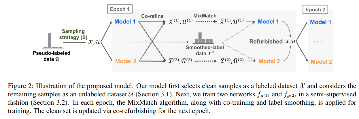
-위의 과정을 정리하면 아래와 같다.

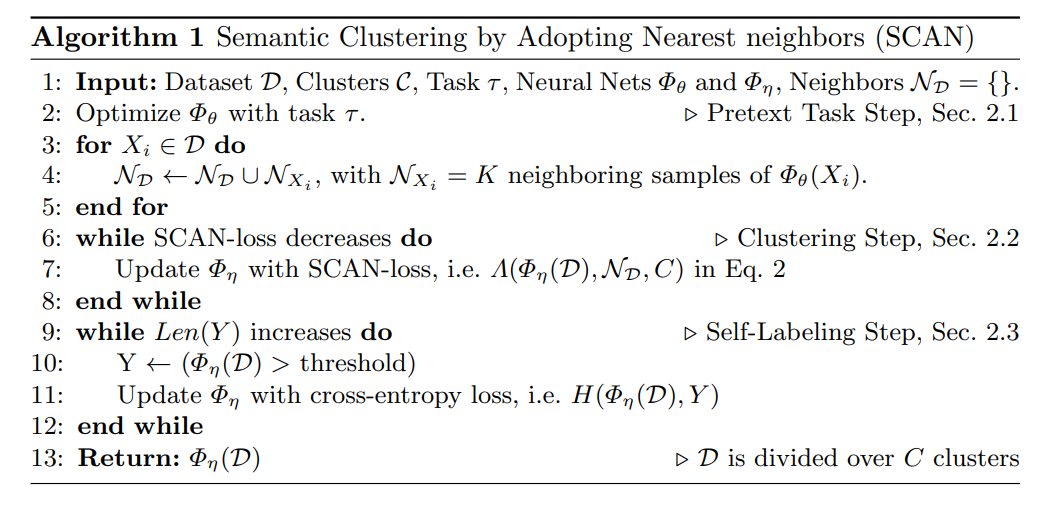
Experiments

* RA - Random Augment

Paper

arxiv.org/abs/1807.06653

Code

github.com/xu-ji/IIC

Introduction

본 논문은 deep-clustering 논문과 같이 simple하게 clustering과 representation learning을 섞은 방법이 degenerate solutions을 만들어 낸다는 문제가 있다는 점을 지적했다.

Invariant Information Clustering (IIC) 방법은 x와 transformation이 적용된 x' sample간의 mutual information을 이용하여 objective function을 구성한 것이 특징이다.

IIC는 다른 method들에 비해 robust한데,

먼저 clustering degeneracy에 대해 robust하다. clustering degeneracy는 cluster의 prediction을 하나의 class로 prediction하는 현상으로 특히 k-means와 representation learning을 조합했을 때, 더 잘 나타난다.

이러한 현상을 IIC에서는 entropy maximisation term을 넣어서 하나의 class로 prediction할 경우 loss값이 커지게 만들어서 해결한다.

두번째는 모델이 label을 잘못 prediction함으로 생기는 noisy data가 발생한다는 것이다. 

이러한 문제를 IIC에서는 auxiliary output layer를 사용함으로 해결한다. 이때 output의 수는 원래 gt의 수보다 더 많게 설정된다. (Auxiliary over-clustering)

Method

IIC는 다음과 같이 x, x'의 representation의 mutual information 값을 maximization하는 방법을 사용한다.

위와 같은 식을 사용하면 x, x'의 representation을 같게 만들어주는 효과가 있다.

위의 mutual information식은 아래와 같이 표현이 가능하다.

위 식을 maximizing하는 것은 다음과 같다.

H(z)를 max로 만드는 것은 z의 확률이 equally하게 형성된다는 것을 의미하며, cluster label assign이 equally하게 되는 것을 의미한다. H(z|z')이 최소화 된다는 것의 의미는 한 sample이 어떤 label로 assign되었을때, 다른 sample도 label이 확정된다는 것을 의미한다. 

이때 , H(z)가 maximize됨으로 cluster degeneration을 막을 수 있다. (하나의 cluster만 형성되는 것을 막을 수 있음)

Paper

arxiv.org/abs/2012.11150

Code

github.com/deu30303/RUC

Introduction

Unsupervised clustering의 경우 많은 연구가 진행되었지만 실제와 다른 label로 misclassified되는 문제가 주요하게 대두되었다. 본 논문에서는 RUC라는 방법을 제안해 이러한 문제를 해결했으며, 이와 같은 noise labeling 문제를 label-smoothing과 co-training으로 접근해 해결한다.

이러한 re-training method는 pseudo-label을 regularize하고 또한 overconfident 문제를 막는다.  

그래서 RUC는 크게 다음과 같은 2개의 key component가 있다.

(1) extracting clean samples

(2) retraining with the refined dataset

- 이를 위해 먼저 confidence값을 이용해 low confidence sample을 걸러낸다.

- 두번째는 metric-based로 non-parametric classifier를 이용해 given instance가 k-nearest sample와 same label을 공유하는지 살펴본다.

- 3번째는 위의 두가지 방법을 combine하여 credible한 sample을 찾아낸다.

그 다음으로는 위와 같은 방식으로 sampled 된 dataset을 이용하여 clustering model을 retraining한다.

MixMatch (badlec.tistory.com/200?category=1015684) 를 이용하며, clean sample을 labeld data, unsample sample을 unlabeled data로 활용한다. 

이때, label smoothing과 block learning을 이용해 denoising effect를 적용한다.

최종적으로 두개의 network를 co-training하는 방법을 사용해서 unclean sample들에 대한 효과를 경감시킨다.

Method

- 먼저 initial clustering의 결과를 noisy-labels 문제로 생각하는 것이 핵심이다.

- 그래서 training을 위해 pseudo-label이 된 데이터를 clean data와 unclean data로 구분하여 생각한다.

- 이때, clean data는 labeled data, unclean data는 unlabeled data로 구분하여 생각하고 이를 semi-supervised 형식으로 재학습하게 된다.

- semi-supervised 방식에서 활용하는 방법은 label smoothing과 co-trainining 방법이다. 

1. Extracting clean samples

- 먼저 trainig sample을 pseudo-label an supervised classifier gΦ을 이용하여 clean data X, unclean data U를 구분한다. 이때 구분하는 기준은 다음과 같이 3가지를 활용한다.

1-1) Confidence-based strategy

- 이 방법은 unsupervised classifier의 confidence score를 기반으로 clean sample을 지정하는 방법이다.

unsupervised classifier가 over-confidence하는 경향이 있기 때문에 threshold를 크게 잡아서 uncertain sample을 최대한 제거하는 방법을 활용한다.

1-2) Metric-based strategy

- Confidence-based 방법은 문제점은 unsupervised classifier의 능력에 의존한다는 점이다. Metric-based 방법은 새로운 embedding network hψ를 활용한다 (SimCLR과 같은 pretext learning 활용). 이때,  hψ(x)의 label은 k-NN 방법을 활용한다. 그리고 최종적으로는 기존 network의 결과 y와 hψ의 kNN based 결과가 같은 경우 clean data라고 판별하고, 아닌 경우 unclean data라고 판별한다.

1-3) Hybrid strategy

- 이 방법의 Confidence, Metric based 방법을 둘다 사용한 것이다.

2. Retraining via Robust Learning

위의 방법을 이용해 clean dataset과 unclean dataset을 구분하면 refine classifier fθ를 학습시킨다. 이때 fθ의 역할은 initial unsupervised classifier의 incorrect prediction들을 correcting 하는 역할이다.

2-1) Semi-supervised learning (MixMatch)

-X와 U가 정해지면 이를 이용해 semi supervied learning을 적용할 수 있다. 이때 사용하는 방법은 MixMatch(badlec.tistory.com/200)이다. 

2-2) Label smoothing

Label Smoothing을 적용함으로 Label Noise를 줄일 수 있다. 때문에 본 논문에서는 semi-supervised learning에 label noise도 함께 적용한다.

(ε은 uniform distribution)

실제로 적용한 방식은 위의 방법으로 생성된 Smoothed label과 RandAugment를 적용한 sample의 ouput에 cross-entropy loss를 적용한다. 

위 loss를 적용한 최종 objective는 다음과 같다.

2-3) Co-training

Network 하나만을 이용하면, 하나의 network가 잘못된 pseudo-label에 over-fitting되는 경우 그 error가 계속해서 그 네트워크에 누적된다는 위험이 존재한다. 이를 막기 위해서 2개의 network를 이용하여 학습을 진행하는 co-training module을 활용한다. 이때 label set X와 unlabel set U에 둘다 co-refinement를 적용한다. labeled data x에 대해서 model 2개의 output을 조합한다.

w(2)는 network 2의 confidence value이다. 

unlabeled set U에 대해서는 아래와 같이 quessing 한다.

m은 augmentation을 의미하며, 여러 augmentation의 결과를 평균내어 나타낸다.

이를 정리하면 다음과 같다.

2-4) Co-refurbishing

마지막으로 학습과정에서 unclean sample중에서 prediction이 확실한 sample들은 clean sample로 추가해준다.

unlabeled data중에서 network를 통과했을때, prediction 확률이 특정 threshold값을 넘는 경우, clean dataset에 추가해준다.

Paper

arxiv.org/abs/2003.08983

Code

github.com/jeromerony/dml_cross_entropy

Introduction

겉으로 보기에는 standard cross-entropy loss와 DML에서 쓰이는 pairwise loss들이 관계가 없어 보인다.

본 논문에서는 실제로는 이 두가지 loss가 관련이 있으며 'MI'(mutual-information)을 통해서 살펴보면 둘다 MI를 최대화하는 방향으로 학습을 시키는 것을 알 수 있다. 그래서 MI를 기반으로 pairwise loss들과 cross-entropy loss는 서로 관련이 있으며 cross-entropy loss는 MI측면에서 upper bound임을 증명한다.

Summary of contributions

1. DML loss들의 관계 및 learned feature와 labels에 대한 MI의 generative view를 정립하였다.

2. standard cross-entropy를 최적화하는 것은 pairwise loss의 bound-optimizer를 approximation하는 것이다. (?)

3. 좀더 제너럴한 뷰에서, standard cross-entropy loss는 discriminative한 뷰에서 feature와 labels간의 MI를 최대화하는 것과 같다.

4. 위와 같은 내용을 실험을 통해 증명하였다.

On the two view of the mutual information

Mutual information은 2개의 random variable이 공유하는 information량을 측정하는 수학적 식이다.

본 논문에서는 learned feature Z와 label Y의 MI를 계산한다. 이때 MI는 대칭이기 때문에 2가지 view로 살펴볼 수 있다.

MI를 maximize 하기 위해서 discriminative view 관점에서 보면 

label은 balanced되어 있어야 하고, ( H(Y)값 최대)  feature가 condition으로 주어진 상황에서는 entropy가 작은, 즉 Y label이 잘 구분되어야 한다. 이와 다르게 generative view는 embedding space상 feature는 최대한 퍼져있어야 하지만 label이 주어졌을 때 feature는 최대한 뭉쳐있어야 함을 의미한다.

이때, discriminative view는 label identification에 집중되어 있고, generative view는 learned feature에 집중되어 있다. 

이는 label 중심의 cross-entropy loss와  feature중심의 feature-shaping loss과의 관계를 분석할 수 있다.

Pairwise losses and the generative view of the MI

Pairwise loss들은 , generative view에서 mutual information을 maximization하는 형태로 해석될 수 있다.

1) The example of contrastive loss

contrastive loss부터 분석을 시작해보자. contrastive loss는 첫번째 항처럼 i,j간의 거리를 줄여주는 term과 ij간의 거리를 특정 margin 이상은 유지하도록 하는 term으로 구성되어 있다. 첫번째 term은 같은 class의 sample간의 거리를 줄여주는 tightness part이고, 두번째 term은 다른 class의 sample 간의 거리를 유지해주는 contrastive part이다.

이때, T_contrast는 다음과 같이 conditional cross entropy로 해석될 수 있다.

이때, center loss 형태이기 때문에 다음과 같이 conditional distribution은 gaussian 분포를 따르게 된다.

이때, T_constant는 다음과 같이 mutual information의 upper bound라고 해석될 수 있다.

이때, Z바|Y는 normal distribution을 따르기 때문에 아래와 같이 Z hat이 normal distribution을 따르면, 이와 같이 tight한 bound를 형성할 수 있고, T_contrast를 minimizing하는 것은 H(Z_hat|Y)를 minimizing하는 것과 같다. 이는 Y가 주어졌을때 Z_hat에 대한 entropy값을 줄이는 것이므로 각 cluster에 대해 feature가 뭉치도록 embedding 시킨다는 것과 같다.

그러나 이러한 형태로 optimization을 진행하는 경우, 모든 data point를 한 곳에 mapping시키는 trivial encoder를 만들어낼 가능성이 있다. 또한 이것이 global optimum이기도 하다. 

이러한 trivial solution을 막기 위해서, second term이 필요하다. 그리고 이 second term이 contrastive term이다. 

이 term은 아래와 같이 구성된다.

그렇기 때문에 D_ij가 m보다 작을때, cost가 발생하고, x를 아래와 같이 정의할때,

다음과 같은 appoximation을 이용해서 식을 고칠 수 있다.

이 식에서 두번째 term은 tightness objective를 만족하기에 충분하다. 

첫번째 term은 differential entropy estimator로 해석이 가능하다. 

2가지 term 모두 Z-hat의 퍼진 정도를 측정한다.  결론적으로 contrastive loss를 minimizing하는 것은 label Y와 embedded feature Z_hat의 MI를 최대화하는 것의 proxy로 해석할 수 있다.

2) Generalizing to other pairwise losses

다른 pairwise loss들도 이와 유사하게 분석이 가능하다.

Cross-entropy does it all

Cross-entropy loss의 경우 위와 같이 tightness part와 contrastive part로 나뉘어지지 않는 것으로 보인다. 

(unary classification loss)

그러나 실제로는 cross-entropy 또한 tightness part와 contrastive part로 나누어 생각할 수 있으며, pairwise loss와 똑같이 MI를 maximization하는 형태로 생각할 수 있다.

아래는 이에 대한 수학적 분석인데, 일단은 생략.. (논문 참고)

1) The pairwise loss behind unary cross-entropy

...

2) A discriminative view of mutual information

...

3) Then why would cross-entropy work better?

저자는 왜 cross-entropy loss와 pairwise loss가 동등하게 MI를 최대화하는 한다고 볼 수 있는데

cross-entropy loss가 더 좋은 성능을 보이는지 간단하게 설명하고 있다.

요약하자만 pairwise loss의 경우, pair를 잘 선정해야 되는 문제에서 부터 다소 복잡한 learning 과정을 수행하는데 반면에 cross-entropy loss는 간단한 형태로 진행되기 때문이라고 말하고 있다.

Paper

openaccess.thecvf.com/content_CVPR_2019/papers/Ye_Unsupervised_Embedding_Learning_via_Invariant_and_Spreading_Instance_Feature_CVPR_2019_paper.pdf

Code

github.com/mangye16/Unsupervised_Embedding_Learning

Method

image를 instance level로 같은 이미지는 가깝게 embedding하고 다른 이미지는 멀리 embedding시킨다.

위 그림은 한 이미지에 augmentation을 적용하기 전 이미지와 후 이미지를 같은 output feature가 나오게 만든다는 의미이다.

이러한 방법을 논문에서는 positive concentrated, negative separated라고 표현한다.

instance-wise한 방법은 general한 feature를 추출하기 때문에 unseen testing categories 구분에도 도움이 된다고 알려져 있다. (Dimensionality Reduction by Learning an Invariant Mapping)

수식은 다음과 같다.

먼저 augmented sample i가 i로 classified 될 확률은 다음과 같다.

sample xj가 instance i로 recognized될 확률은 다음과 같다.

그래서 augmented sample i 가 i로 classifed되고 j로 prediction되지 않을 확률은 다음과 같다.

이 수식에 대한 negative log likelihood를 계산하면,

이를 batch내에 있는 모든 instance에 대해서 계산하면 다음과 같다.

또한 training을 위해서 Siamese Network를 사용한다.

augmented sample의 feature를 뽑기 위함이며, 상세한 사항은 위 그림을 참고하면 된다.

Results

Paper

openaccess.thecvf.com/content_cvpr_2018/CameraReady/0801.pdf

Code

github.com/zhirongw/lemniscate.pytorch

Introduction

Imagenet dataset을 기존의 supervised learning 형태로 학습시키게 되면 위와 같이 input image에 대해 유사한 class들이 softmax output에서 높은 값을 나타내는 것을 확인할 수 있다. 

이는 일반적인 supervised learning이 class별로 annotation을 하여 학습시키기는 하지만 결과적으로 image간의 유사성을 스스로 학습할 수 있다는 의미를 나타낸다.

이러한 결과를 토대로 본 논문에서는 class-wise learning을 instance-wise learning 형태로 변형하여 시도한다. 

Can we learn a meaningful metric that reflects apparent similarity among instances via pure discriminative learning?

그러나 이러한 방법을 사용할 경우, imagenet dataset 기준으로 class의 수가 1000개에서 1.2 million개로 늘어나게 된다.

단순히 softmax를 이용해서는 이러한 class수를 다루기 어렵기 때문에, NCE 및 proximal regularization 방법을 활용한다.

이전 논문의 경우 umsupervised learning을 통해 feature learning을 수행하면 SVM과 같은 linear classifier를 통해 classification을 수행했다.

그러나 SVM과 같은 linear classifier가 동작을 잘한다는 보장은 없다.

본 논문에서는 non-parametric한 방법인 kNN classification 방법을 사용한다.

이때, test time마다 거리 계산을 위해 training sample을 모두 embedding 시킬 수는 없기 때문에 

memory bank를 활용하여 training sample을 embedding 시킨 값을 저장해놓는다.

(일반적인 classifier는 거리 계산을 위해 각 class의 대표값만을 저장해두는데, 그것이 weight이다.)

Non-parametric classifier

1) parametric classifier

일반적으로 사용하는 parametric classifier

2) Non-parametric Classifier

parametric과 다르게 instance 별로 진행한다. 

이때 , v 벡터는 normalization을 적용하며, 아래와 같이 거리 기반으로 계산할 때, 유사한 class끼리 더 가깝게 embedding 되는 효과를 얻을 수 있다.

Noise-Contrastive Estimation

class수가 매우 많은 경우, softmax 계산이 어려워진다. 이와 같은 문제는 word embedding에서도 발생했었고 다음과 같이 해결 했다.

• Hierarchical Softmax: 각 단어들을 leaves로 가지는 binary tree를 하나 만들고, 해당하는 단어의 확률을 계산할 때 root에서부터 해당 leaf로 가는 길을 따라 확률을 곱해 해당 단어가 나올 최종적인 확률을 계산한다.자세한 설명은 위 그림 클릭

• 

• Negative Sampling : 모든 단어들에 대해 Softmax를 수행하므로 계산량이 많아지는 것을 개선하기 위해 해당하는 단어와 그렇지 않은 일정 개수의 Negative Sample에 대해 Softmax를 수행한다.
• Noise-Contrastive Estimation : multi-class classification을 data sample인지 noise sample인지 판단하는 binary classification으로 바꾼다.

본 논문에서는 NCE를 사용한다. feature v를 가지는 입력 i가 data sample일 posterior probability은 다음과 같다.

• Pn=1/n : noise distribution
• mPn : noise sample이 data sample보다 mm배 더 많다고 가정

이를 통해 만들어지는 objective function은 다음과 같다.

• Pd : actual data distribution
• v′ : Pn에서 무작위로 sampling된 이미지들의 representation

이때,  Zi의 계산량이 여전히 많으므로 이를 Monte Carlo 근사를 이용해 계산량을 줄인다.

(  {jk} : 무작위 인덱스의 집합, V가 계산되지 않은 첫번째 iteration에도 근사는 유효했음  )

Proximal Regularization

일반적인 classification과 달리 본 논문은 한 class당 하나의 이미지만 가지고 학습한다. 따라서 각 epoch당 각 class는 한 번만 학습되고 매번 loss가 크게 진동한다. 이를 완화하기 위해 regularization term을 추가한다.

Weighted k-Nearest Neighbor Classifier

Parametric vs. Non-parametric So

ftmax

Image Classification

Qualitative case study

Paper

arxiv.org/abs/1901.04596

Code

github.com/maple-research-lab/AET

AET: The Proposed Approach

특정한 transformation을 이용해 image를 변환하고 변환 전 image x 와 변환 후 image t(x)를 encoding한다. 

이를 이용해 decoding하여 transformation을 예측하게 하고, 실제 transformation t와 예측된 transformation t(hat)

을 비교하여 loss-function을 구성한다.

Paper

arxiv.org/abs/1910.05872

Code

github.com/hankook/SLA

Introduction

그동안의 self-supervised task를 이용한 방법은 multi-task learning의 형태가 많았다.

(Multi task learning은 아래 그림 참고) 

그러나 multi task learning 방식은 단순히 supervised 방식을 사용했을 때 보다 acc gain은 없다. 

그렇다면 어떻게 self-supervision을 fully supervised classfication task에 적용하는 것이 가장 좋은 방법일까? 

Contribution

먼저 multi task learning의 경우 primary network에 대해서 self-supervision task (transformation)에 대해서 invariant하게 만든다. 예를들어 Rotnet의 경우 rotation에 대해 invariant하게 만들어주는 방식이다.

그러나 이러한 invariance는 오히려 task에 대한 난이도 및 복잡도를 증가시킬 수 있다.

예를들어 {6 vs 9} 와 {bird vs bat} 같은 경우 회전때문에 오히여 두 클래스가 더 헷갈릴수도 있기 때문이다.

그리고 이러한 이유 때문에 오히려 multi-task learning이 성능이 더 저하되는 경우가 생긴다.

(아래 그림 baseline과 MT(Multi-Task) accuracy 비교)

이러한 문제를 해결하기 위해서, 저자들은 기존의 label과 self-supervision label을 조합한 joint distribution을 제안한다.

예를들어 cifar10 dataset과 Rotnet을 조합하는 경우 10 label * 4label (0, 90, 180, 270) 총 40 label이다. 

이렇게 하면 multi task learning의 경우 class에 대한 label 없이 Rotation에 해당하는 label을 맞추어야 하기 때문에 오히려 classificaition 성능이 떨어지는 상황이 발생하나, joint의 경우 각 input으로 들어오는 image가 어떤 class에 대한 정보를 rotation과 함께 부여하기 때문에 이러한 문제가 해결할 수 있다.

또한 아래 그림과 같이 특정 class에 대한 self-supervision prediction에 대한 결과들을 aggregation하여 앙상블 효과 또한 얻을 수 있다. 

본 논문에서는 self_supervision task로서 Rotation과 Color Permutation 방법을 사용했으며, fully-supervised, few-shot, imbalanced dataset에서 성능향상을 볼 수 있었다.

Self-supervised Label Augmentation

* notation

input :

label : (N은 class의 수)

cross entropy loss function:

softmax classifier :

embedding vector of x :

augmented sample using transformation t 

the embedding of the augmetnted sample x:

Aggregated inference

label을 joint하여 learning한 이후에 inference의 경우는 다음과 같이 한다.

class에 해당하는 self-supervision transformation의 logit을 모두 더한다.

그렇게 하면 class별 logit이 새롭게 산출되고 이를 softmax를 이용해서 prediction한다.

이러한 방식은 앙상블 방식으로 해석할 수 있는데, 

실제로 independent한 여러개의 모델을 앙상블 한 것 보다 더 높은 성능이 나왔다.

Self-distillation from aggregation

aggrregation이 성능향상에 큰 도움을 주기는 하지만, inference과정에서 기존의 label보다 훨씬 많은 label에 대한 

summation 계산과정이 있기 때문에, computation cost가 존재한다. 

이러한 inference과정에서 computational cost를 줄이기 위해서 본 논문에서는 self-distillation방법을 사용한다. 

그래서 aggregated된 knowledge

를 다른 classifier에 distillation한다.(그림참고)

즉 feature extractor에 n*m (label 개수 10*4)의 classifier와 n(label 개수 10) classifier 2개를 놓고, n*m classifier는 label을 통해 학습시키고 n classifier의 경우, distilation을 통해 학습시킨다.

그리고 inference 단계에서는 self-distilation을 통해 학습된 classifier를 이용해 inference한다.

최종적인 loss function은 다음과 같다.

Comparison with DA and MT

본 논문에서는 data-augmentation과 Self-supervised Multi-task learning이 유사한 성격을 지닌다고 주장하고 있다.

또한 rotation 기반으로 생각했을 때, unnecessary한 invariant 속성을 학습하기 때문에 오히려 성능이 떨어진다고 주장한다. 

이때, test에 대해서 DA와 MT가 낮은 것은 앞선 unnecessary한 부분을 invariant하게 만들기 때문이다.

MT가 train 및 test 모두 성능이 안좋은 이유는 optimization 자체가 hard하기 때문이라고 말하고 있다.

위의 그래프에 대한 성능은 아래와 같다.  

이때 DA가 Baseline보다도 성능이 낮은데, 둘의 차이는 rotation based augmentation이 있냐 없냐의 차이이다.

내 생각엔 Baseline에 다른 augmentation이 분명 포함되어 있을거라고 생각한다.

Imbalanced classification

Imbalanced classification에도 큰 성능향상을 보임 (왜?)