Learning to Learn

Paper

arxiv.org/abs/2003.08983

Code

github.com/jeromerony/dml_cross_entropy

Introduction

겉으로 보기에는 standard cross-entropy loss와 DML에서 쓰이는 pairwise loss들이 관계가 없어 보인다.

본 논문에서는 실제로는 이 두가지 loss가 관련이 있으며 'MI'(mutual-information)을 통해서 살펴보면 둘다 MI를 최대화하는 방향으로 학습을 시키는 것을 알 수 있다. 그래서 MI를 기반으로 pairwise loss들과 cross-entropy loss는 서로 관련이 있으며 cross-entropy loss는 MI측면에서 upper bound임을 증명한다.

Summary of contributions

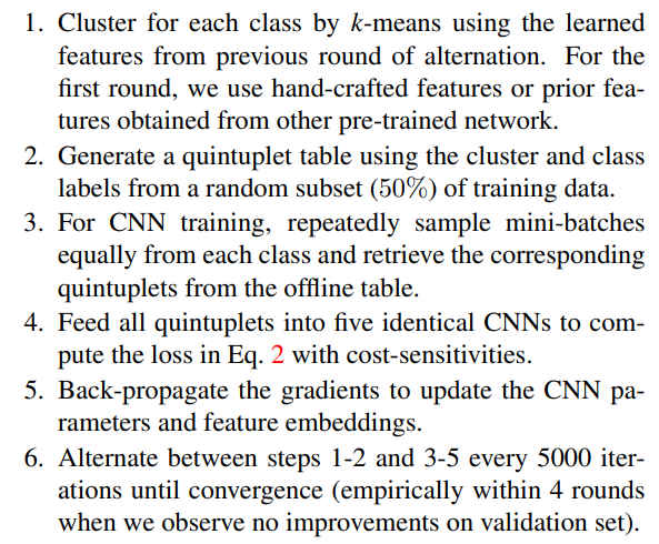
1. DML loss들의 관계 및 learned feature와 labels에 대한 MI의 generative view를 정립하였다.

2. standard cross-entropy를 최적화하는 것은 pairwise loss의 bound-optimizer를 approximation하는 것이다. (?)

3. 좀더 제너럴한 뷰에서, standard cross-entropy loss는 discriminative한 뷰에서 feature와 labels간의 MI를 최대화하는 것과 같다.

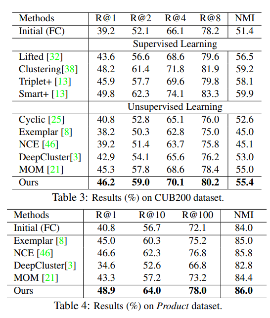
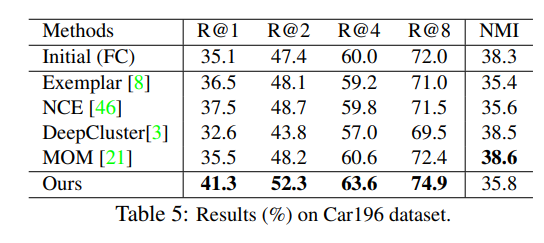
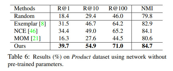
4. 위와 같은 내용을 실험을 통해 증명하였다.

On the two view of the mutual information

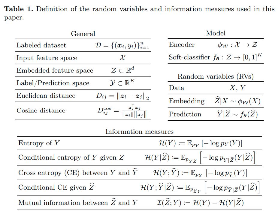
Mutual information은 2개의 random variable이 공유하는 information량을 측정하는 수학적 식이다.

본 논문에서는 learned feature Z와 label Y의 MI를 계산한다. 이때 MI는 대칭이기 때문에 2가지 view로 살펴볼 수 있다.

MI를 maximize 하기 위해서 discriminative view 관점에서 보면 

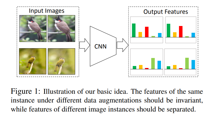
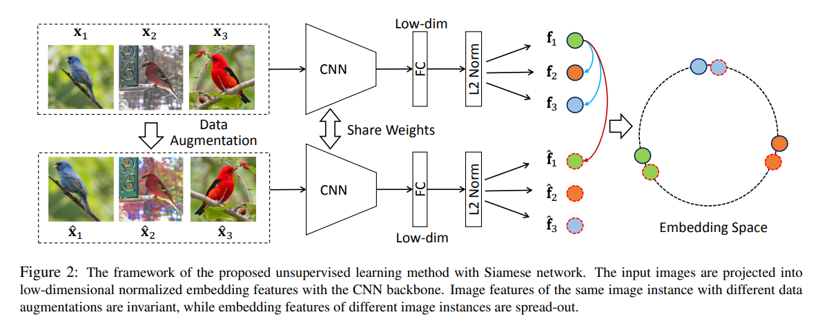
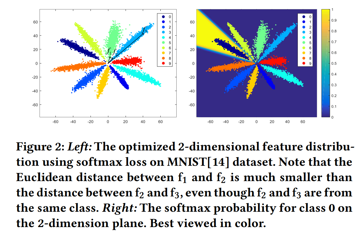
label은 balanced되어 있어야 하고, ( H(Y)값 최대)  feature가 condition으로 주어진 상황에서는 entropy가 작은, 즉 Y label이 잘 구분되어야 한다. 이와 다르게 generative view는 embedding space상 feature는 최대한 퍼져있어야 하지만 label이 주어졌을 때 feature는 최대한 뭉쳐있어야 함을 의미한다.

이때, discriminative view는 label identification에 집중되어 있고, generative view는 learned feature에 집중되어 있다. 

이는 label 중심의 cross-entropy loss와  feature중심의 feature-shaping loss과의 관계를 분석할 수 있다.

Pairwise losses and the generative view of the MI

Pairwise loss들은 , generative view에서 mutual information을 maximization하는 형태로 해석될 수 있다.

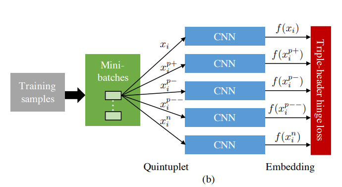
1) The example of contrastive loss

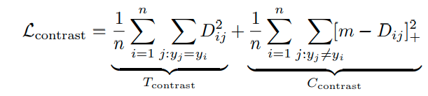
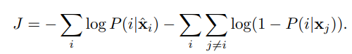
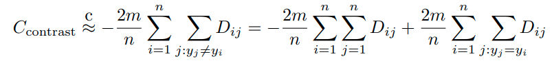
contrastive loss부터 분석을 시작해보자. contrastive loss는 첫번째 항처럼 i,j간의 거리를 줄여주는 term과 ij간의 거리를 특정 margin 이상은 유지하도록 하는 term으로 구성되어 있다. 첫번째 term은 같은 class의 sample간의 거리를 줄여주는 tightness part이고, 두번째 term은 다른 class의 sample 간의 거리를 유지해주는 contrastive part이다.

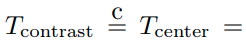
이때, T_contrast는 다음과 같이 conditional cross entropy로 해석될 수 있다.

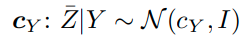
이때, center loss 형태이기 때문에 다음과 같이 conditional distribution은 gaussian 분포를 따르게 된다.

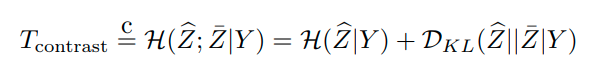
이때, T_constant는 다음과 같이 mutual information의 upper bound라고 해석될 수 있다.

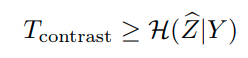
이때, Z바|Y는 normal distribution을 따르기 때문에 아래와 같이 Z hat이 normal distribution을 따르면, 이와 같이 tight한 bound를 형성할 수 있고, T_contrast를 minimizing하는 것은 H(Z_hat|Y)를 minimizing하는 것과 같다. 이는 Y가 주어졌을때 Z_hat에 대한 entropy값을 줄이는 것이므로 각 cluster에 대해 feature가 뭉치도록 embedding 시킨다는 것과 같다.

그러나 이러한 형태로 optimization을 진행하는 경우, 모든 data point를 한 곳에 mapping시키는 trivial encoder를 만들어낼 가능성이 있다. 또한 이것이 global optimum이기도 하다. 

이러한 trivial solution을 막기 위해서, second term이 필요하다. 그리고 이 second term이 contrastive term이다. 

이 term은 아래와 같이 구성된다.

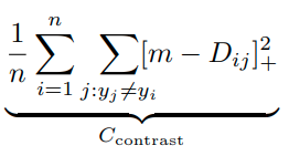
그렇기 때문에 D_ij가 m보다 작을때, cost가 발생하고, x를 아래와 같이 정의할때,

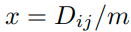
다음과 같은 appoximation을 이용해서 식을 고칠 수 있다.

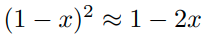
이 식에서 두번째 term은 tightness objective를 만족하기에 충분하다. 

첫번째 term은 differential entropy estimator로 해석이 가능하다. 

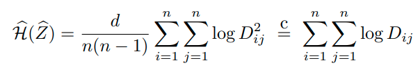
2가지 term 모두 Z-hat의 퍼진 정도를 측정한다.  결론적으로 contrastive loss를 minimizing하는 것은 label Y와 embedded feature Z_hat의 MI를 최대화하는 것의 proxy로 해석할 수 있다.

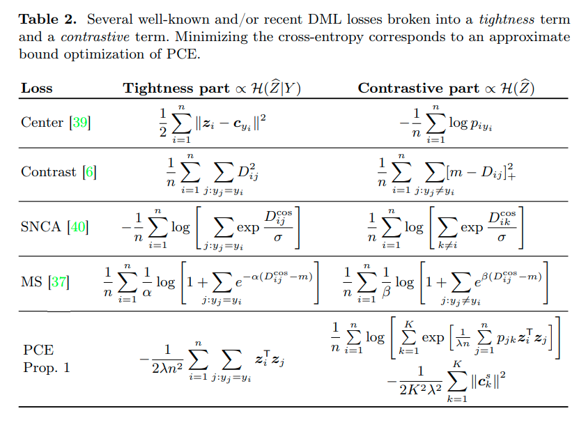
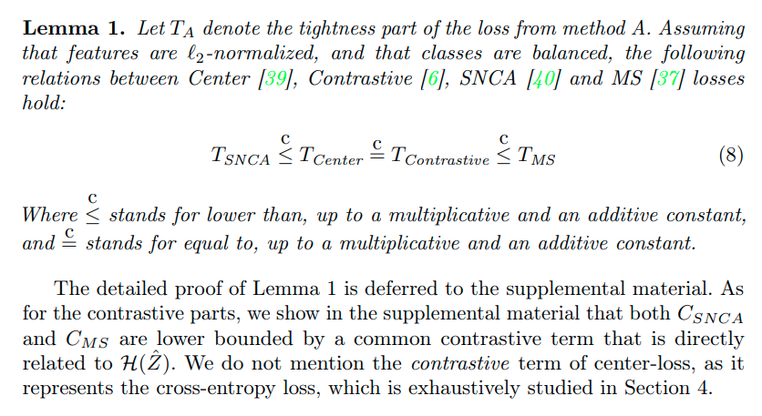
2) Generalizing to other pairwise losses

다른 pairwise loss들도 이와 유사하게 분석이 가능하다.

Cross-entropy does it all

Cross-entropy loss의 경우 위와 같이 tightness part와 contrastive part로 나뉘어지지 않는 것으로 보인다. 

(unary classification loss)

그러나 실제로는 cross-entropy 또한 tightness part와 contrastive part로 나누어 생각할 수 있으며, pairwise loss와 똑같이 MI를 maximization하는 형태로 생각할 수 있다.

아래는 이에 대한 수학적 분석인데, 일단은 생략.. (논문 참고)

1) The pairwise loss behind unary cross-entropy

...

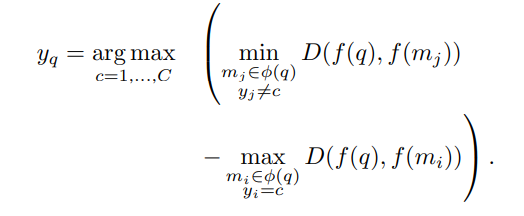
2) A discriminative view of mutual information

...

3) Then why would cross-entropy work better?

저자는 왜 cross-entropy loss와 pairwise loss가 동등하게 MI를 최대화하는 한다고 볼 수 있는데

cross-entropy loss가 더 좋은 성능을 보이는지 간단하게 설명하고 있다.

요약하자만 pairwise loss의 경우, pair를 잘 선정해야 되는 문제에서 부터 다소 복잡한 learning 과정을 수행하는데 반면에 cross-entropy loss는 간단한 형태로 진행되기 때문이라고 말하고 있다.

Paper

openaccess.thecvf.com/content_CVPR_2019/papers/Ye_Unsupervised_Embedding_Learning_via_Invariant_and_Spreading_Instance_Feature_CVPR_2019_paper.pdf

Code

github.com/mangye16/Unsupervised_Embedding_Learning

Method

image를 instance level로 같은 이미지는 가깝게 embedding하고 다른 이미지는 멀리 embedding시킨다.

위 그림은 한 이미지에 augmentation을 적용하기 전 이미지와 후 이미지를 같은 output feature가 나오게 만든다는 의미이다.

이러한 방법을 논문에서는 positive concentrated, negative separated라고 표현한다.

instance-wise한 방법은 general한 feature를 추출하기 때문에 unseen testing categories 구분에도 도움이 된다고 알려져 있다. (Dimensionality Reduction by Learning an Invariant Mapping)

수식은 다음과 같다.

먼저 augmented sample i가 i로 classified 될 확률은 다음과 같다.

sample xj가 instance i로 recognized될 확률은 다음과 같다.

그래서 augmented sample i 가 i로 classifed되고 j로 prediction되지 않을 확률은 다음과 같다.

이 수식에 대한 negative log likelihood를 계산하면,

이를 batch내에 있는 모든 instance에 대해서 계산하면 다음과 같다.

또한 training을 위해서 Siamese Network를 사용한다.

augmented sample의 feature를 뽑기 위함이며, 상세한 사항은 위 그림을 참고하면 된다.

Results

Paper

openaccess.thecvf.com/content_cvpr_2018/CameraReady/0801.pdf

Code

github.com/zhirongw/lemniscate.pytorch

Introduction

Imagenet dataset을 기존의 supervised learning 형태로 학습시키게 되면 위와 같이 input image에 대해 유사한 class들이 softmax output에서 높은 값을 나타내는 것을 확인할 수 있다. 

이는 일반적인 supervised learning이 class별로 annotation을 하여 학습시키기는 하지만 결과적으로 image간의 유사성을 스스로 학습할 수 있다는 의미를 나타낸다.

이러한 결과를 토대로 본 논문에서는 class-wise learning을 instance-wise learning 형태로 변형하여 시도한다. 

Can we learn a meaningful metric that reflects apparent similarity among instances via pure discriminative learning?

그러나 이러한 방법을 사용할 경우, imagenet dataset 기준으로 class의 수가 1000개에서 1.2 million개로 늘어나게 된다.

단순히 softmax를 이용해서는 이러한 class수를 다루기 어렵기 때문에, NCE 및 proximal regularization 방법을 활용한다.

이전 논문의 경우 umsupervised learning을 통해 feature learning을 수행하면 SVM과 같은 linear classifier를 통해 classification을 수행했다.

그러나 SVM과 같은 linear classifier가 동작을 잘한다는 보장은 없다.

본 논문에서는 non-parametric한 방법인 kNN classification 방법을 사용한다.

이때, test time마다 거리 계산을 위해 training sample을 모두 embedding 시킬 수는 없기 때문에 

memory bank를 활용하여 training sample을 embedding 시킨 값을 저장해놓는다.

(일반적인 classifier는 거리 계산을 위해 각 class의 대표값만을 저장해두는데, 그것이 weight이다.)

Non-parametric classifier

1) parametric classifier

일반적으로 사용하는 parametric classifier

2) Non-parametric Classifier

parametric과 다르게 instance 별로 진행한다. 

이때 , v 벡터는 normalization을 적용하며, 아래와 같이 거리 기반으로 계산할 때, 유사한 class끼리 더 가깝게 embedding 되는 효과를 얻을 수 있다.

Noise-Contrastive Estimation

class수가 매우 많은 경우, softmax 계산이 어려워진다. 이와 같은 문제는 word embedding에서도 발생했었고 다음과 같이 해결 했다.

• Hierarchical Softmax: 각 단어들을 leaves로 가지는 binary tree를 하나 만들고, 해당하는 단어의 확률을 계산할 때 root에서부터 해당 leaf로 가는 길을 따라 확률을 곱해 해당 단어가 나올 최종적인 확률을 계산한다.자세한 설명은 위 그림 클릭

• 

• Negative Sampling : 모든 단어들에 대해 Softmax를 수행하므로 계산량이 많아지는 것을 개선하기 위해 해당하는 단어와 그렇지 않은 일정 개수의 Negative Sample에 대해 Softmax를 수행한다.
• Noise-Contrastive Estimation : multi-class classification을 data sample인지 noise sample인지 판단하는 binary classification으로 바꾼다.

본 논문에서는 NCE를 사용한다. feature v를 가지는 입력 i가 data sample일 posterior probability은 다음과 같다.

• Pn=1/n : noise distribution
• mPn : noise sample이 data sample보다 mm배 더 많다고 가정

이를 통해 만들어지는 objective function은 다음과 같다.

• Pd : actual data distribution
• v′ : Pn에서 무작위로 sampling된 이미지들의 representation

이때,  Zi의 계산량이 여전히 많으므로 이를 Monte Carlo 근사를 이용해 계산량을 줄인다.

(  {jk} : 무작위 인덱스의 집합, V가 계산되지 않은 첫번째 iteration에도 근사는 유효했음  )

Proximal Regularization

일반적인 classification과 달리 본 논문은 한 class당 하나의 이미지만 가지고 학습한다. 따라서 각 epoch당 각 class는 한 번만 학습되고 매번 loss가 크게 진동한다. 이를 완화하기 위해 regularization term을 추가한다.

Weighted k-Nearest Neighbor Classifier

Parametric vs. Non-parametric So

ftmax

Image Classification

Qualitative case study

ddiri01.tistory.com/310

jangun.com/study/StatisticsConceptProblem.html

- 제프리스의 사전분포 검색

en.wikipedia.org/wiki/Kernel_(statistics)

Paper

arxiv.org/abs/1910.09217

Code

github.com/facebookresearch/classifier-balancing

Abstract

다음과 같은 2가지 현상을 발견하였다.

1) data imbalanced learning은 high-quality representation learning 문제가 아닐 수 있다.

2) 가장 단순한 instance-balanced sampling을 통한 representation learning과 더불어 classifier만 adjusting하는 것이 가장 좋은 성능을 보일 수 있다.

Introduction

기존의 방법들은 representation과 classifirer를 따로 분리하지 않고 joint learning을 수행하였다. 

그러나 이러한 방법들은 imbalanced learning에 대한 성능 향상이 어디서 오는 것인지 알 수 없다는 단점이 있다.

그래서 본 논문에서는 representation learning과 classifirer learning을 decoupled해서 분석한다.

representation learning을 비교하기 위해 다음과 같이 3가지 방법을 사용하고 비교해본다.

1) instance-based sampling

2) class-balanced sampling

3) mixture of them

classifier learning을 비교하기 위해 다음과 같이 3가지 방법을 사용하고 비교해본다.

1) re-training the parametric linear classifier in class-balancing manner

2) non-parametric nearest class mean classifier: which classifies the data based on their closest class-specific mean representations from the training set

3) normalizing the classifier weights, which adjusts the weight magnitude directly to be more balanced, adding a temperature to modulate the normalization procedure.

Method

- Sampling strategies

Sampling은 아래와 같이 class당 sampling될 확률을 정의함으로서, 수행되어진다.

이때, q는 sampling 전략을 나타내는 변수이며, 1, 0, 1/2 중 하나의 값을 가진다.

1) Instance-balanced sampling

q=1 일때 instance-balanced sampling을 수행하게 된다. class당 가지고 있는 sample의 수에 비례하여 

sampling을 수행하게 된다.

2) Class-balanced sampling 

q=0 일때, 이며, class당 sampling하는 확률을 모두 동일하게 가져가는 전략이다.

3) Square root sampling

q=1/2이며, sample의 수의 squre root에 비례하여 sampling하는 기법이다. 

4) progressively-balanced sampling

본 방법은 Instance-balanced sampling과 Class-balanced sampling을 혼합한 방법이다.

초반 epoch에는 instance-balanced 기반으로 sampling을 진행하다가 일정 epoch이후에는 class-balanced 형태로

변형되는 sampling기법이다. 자세한 수식은 위와 같다.

- Loss re-weighting strategies

focal-loss, LDAM loss가 대표적으로 있다.

Classification for long-tailed recognition

1) Classifier Re-training (cRT)

representation learning 부분을 fixed하고 classifier만 class balanced 형식으로 다시 학습시키는 방법을 말한다.

2) Nearest Class Mean classifier (NCM)

먼저 각 train data의 class의 mean feature representation을 구한 다음, 이후 query vector의 L2 normalized feature를 활용해서 cosine similarity나 Euclidean distance를 이용해서 nearest neighbor search를 수행한다.

3) τ-normalized classifier 

-instance-balanced sampling의 경우, weight값이 class sample 수에 비례하는 것을 확인할 수 있다.

(sample수가 많은 class의 경우 더 넓은 boundary를 가지게 되고, 이것이 weight값의 크기로 나타남)

-class-balanced sampline의 경우, class마다 sample수가 동일하기 때문에 weight의 값이 class마다 비슷하게 형성되는 것을 확인할 수 있다. (decision boundary가 유사해짐.)

- τ-normalization은 이 2가지 방법의 중간 정도의 방법이다. instance-balanced sampling의 weight에다가 normalization을 하여 'smoothing'한다.

이때 τ는 0~1 사이에서 결정된다.

- Learnable weight scaling (LWS)

scaling하는 정도는 학습을 통해서 얻는 방법을 의미.

Experiment

-Sampling strategies and decoupled learning

- joint training scheme

classifier와 representation learning이 함께 이루어지는 방식이다. 90 epoch 동안 cross-entropy loss 및 instance-balanced, Class-balanced, Square-root, Progressively-balanced.  

- decoupled learning schemes

 classifier만 다시 training 한다. cRT , NCM, τ-normalized classifier가 사용된다. 

먼저 joint의 경우 더 나은 balanced 방법을 적용할 수록 성능이 향상되는 것을 확인할 수 있다.

(joint 부분만 보면서 세로로 분석하면 됨)

decoupled learning을 하는 경우, non-parametric 방법인 NCM을 적용한 경우라도 오히려 성능이 크게 향상되는 것을 볼 수 있다. parametric한 방법은 더욱 성능이 향상 된다. (가로축으로 성능 변화 살펴보면 됨)

여기서 중요한 발견 중 하나는 representation learning에 있어서 instance smapling이 가장 성능이 높다는 것이다.

이는 data-imbalanced issue는 high-quality representation을 배우는데 상관이 없음을 알려준다. 

위 그림은 각 방법에 대한 decision boundary 형성을 그림으로 나타낸 것이다. 

τ 가 0 인 경우는 normalization을 전혀하지 않은 경우이고,  sample수에 비례해서 decision boundary도 정해지기 때문에 더 많은 sample을 가진 class가 더 넓은 decision boundary를 지님을 알 수 있다. τ가 1인 경우에는 normalization이 적용되기 때문에 좀 더 balanced된 boundary가 형성된다. Cosine 같은 경우 모두 같은 크기의 boundary가 형성된다. 마지막은 각 class마다 mean을 구하고 L2로 nearest neighbor 형태로 classifying을 할때, 나타나는 decision boundary를 나타낸 것이다.

results

Paper

openaccess.thecvf.com/content_cvpr_2016/papers/Huang_Learning_Deep_Representation_CVPR_2016_paper.pdf

Method

imbalanced problem의 근본적인 문제점은 minority class를 학습하기 위한 sample이 부족하다는 것인데, minority class에 대해서 4개의 anchor를 설정함으로 majority class에 비해 더 많은 학습 및 embedding을 형성하도록 하는 방법이다.

먼저 embedding 공간을 L2-norm이 1로 제한된 공간에 놔둔다.

- Quintuplet Sampling

quintuplet은 다음과 같이 정의된다. (그림 참고)

이를 통해 다음과 같이 거리를 설정한다. (위 그림 참고)

이러한 quintuplet method는 2가지 메리트가 있다.

1) Triplet loss는 단순히 같은 class끼리는 당기고 다른 class는 떨어트리는 방식을 사용한다. 그러나 quintuplet은 class간과 class 내부의 instance level까지 같이 고려하기 때문에 더 rich한 feature를 추출할 수 있다는 장점이 있다. 

2) under sampling 방법과 비교하면 information loss가 없고, over-sampling과 비교하면 주로 사용되는 artifitial noise가 없다는 장점이 있다. 실제 구현에서는 mini-batch에 minority class와 majority class 같은 숫자를 넣고 학습을 시킨다.

실제 구현에서 quintuplet을 선정하기 위해서는 이미 위 그림의 cluster들의 초기 형태가 형성되있어야 한다.

그래서 특정 데이터셋에서 pre-trained된 모델을 사용하여 feature를 추출하고 이를 통해 k-means clustering을 하여 cluster를 형성한다.

이러한 clustering을 좀 더 robust하게 하기 위해 5000 iteration마다 cluster 형성을 새롭게 업데이트 한다.

- Triple-Header Hinge Loss

위의 그림을 loss function형태로 구현 한 것이다. (잘 모르겠으면 margin loss 참고)

이와 같이 loss를 구현하면 실제로는 아래와 같이 embedding space가 구현된다.

learning하는 방식은 다음과 같다.

실제 학습할 때는 look-up table (dictionary 형태로 거리 저장한다는 의미인듯) 그리고 hardest한 학습은 피하기 위해서 실제 training set에서 50%만 random으로 sampling하여 사용한다. 

요약하면 다음과 같다.

- Difference between "Quintuplet" Loss and Triplet Loss

Triplet Loss의 경우 class기반으로 같은 class 끼리는 뭉치게 만들고 다른 class sample끼리는 멀리 떨어지게 만들기 때문에, 실제 imbalanced data의 문제인 적은 sample 수를 가진 class의 적절한 boundary 혹은 margin을 표현하지 못할 수 있다. (실제로는 더 넓은 지역을 cover해야 하지만, few sample로는 넓은 지역을 다 cover 못할 수 있음)

이에 반해 Quintuplet의 경우, class 내부에 또 다른 cluster를 형성하며, 이는 class 내부에서 생기는 variance를 표현할 수 있다. 이를 통해서 좀 더 넓은 class의 margin 및 boundary를 형성할 수 있고. imbalance에서 생기는 적절한 boundary를 형성하는 문제에서 도움이 될 수 있다.

- Nearset Neighbor Imbalanced Classfication 

본 논문에서는 Classification을 위해서 kNN Classification 방법을 사용한다. 

기존 kNN과 차이점은 다음과 같다. 

1) 기존 knn은 sample-wise로 classificaiton을 하였지만, 본 논문에서는 class마다 형성된 cluster-wise로 knn을 수행한다.

2) Classificaiton을 위해 다음과 같은 공식을 함께 이용한다.

요약하자면 assumtion 하는 class에 해당하는 가장 멀리있는 cluster와의 거리와 해당 class를 제외한 나머지 class의 cluster중에서 가장 가까운 거리를 계산해 차이를 구한다. 이때, 위 식의 값이 크다는 말은, 특정 class에 해당하는 cluster와를 max값을 취했는데도 작다. 즉, 가깝다는 의미이고, 특정 class를 제외한 class들과의 거리 중에서 가장 작은 값을 취했는데도 크다. 즉, 다른 class들과는 멀다는 의미이므로, 특정 class에 query가 가장 가깝다고 할 수 있다.

이러한 방식은 다음과 같은 장점이 있다.

1) imbalanced 환경에 더 강건하다:

기존 방법의 경우 가장 가까운 class의 개수를 통해서만 prediction하기 때문에 imbalanced 문제를 해결하기 힘드나 본논문에서 제시한 embedding 방법과 위의 classicification rule을 함께 적용하면, minority class에 대해서도 large margin을 가져갈 수 있기 때문에 강건한 결과를 낳는다.

2) cluster wise search를 수행하기 때문에 속도가 sample-wise에 비해 빠르다.

결론적으로 실제 동작하는 순서는 다음과 같다.