728x90
728x90
'Dic' 카테고리의 다른 글
| ML & MAP (0) | 2021.03.04 |
|---|---|
| Fov (Field of View) (0) | 2021.02.22 |
| Sampling with replacement (0) | 2021.01.07 |
| Bayes optimal classifier (0) | 2021.01.04 |
| Gaussian mixture model (0) | 2021.01.01 |
| ML & MAP (0) | 2021.03.04 |
|---|---|
| Fov (Field of View) (0) | 2021.02.22 |
| Sampling with replacement (0) | 2021.01.07 |
| Bayes optimal classifier (0) | 2021.01.04 |
| Gaussian mixture model (0) | 2021.01.01 |
Paper :arxiv.org/abs/1911.05722
Momentum Contrast for Unsupervised Visual Representation Learning
We present Momentum Contrast (MoCo) for unsupervised visual representation learning. From a perspective on contrastive learning as dictionary look-up, we build a dynamic dictionary with a queue and a moving-averaged encoder. This enables building a large a
arxiv.org
Code :github.com/facebookresearch/moco
facebookresearch/moco
PyTorch implementation of MoCo: https://arxiv.org/abs/1911.05722 - facebookresearch/moco
github.com
Introduction
MoCo는 Contrasive learning 기반 unsupervised learninig method로서 contrasive learning 적용을 위한 'key' sample을 queue형태로 구성하고, key sample 용도의 encoder를 moving average 형태로 update하는 방식이다.
그래서 아래와 같은 형태를 띈다.
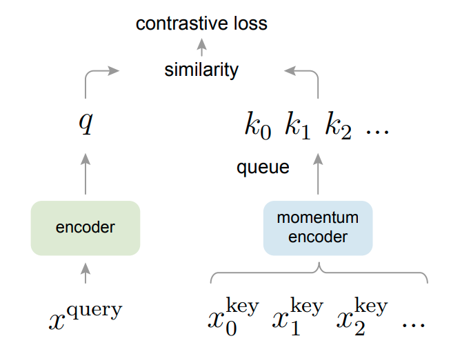
기존의 contrasive learning과 가장 크게 다른 점은 key sample들을 queue형태로 저장한다는 점이다.
그래서 현재의 mini-batch에 있는 sample들은 encoding되어 enqueue되면, oldest는 dequeue된다.
이러한 queue memory를 사용하는 경우, dictionary size를 mini-batch size 이상으로 크게 키울 수 있다는 장점이 있다.
게다가 이전의 key를 저장하고 사용할 수 있기 때문에, key encoder의 변화를 'slowly progressing' 할 수 있다.
이러한 방법을 통해 key encoder가 생성하는 feature의 consistency를 유지할 수 있다.
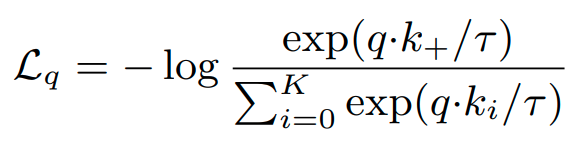
Contrastive Learning as Dictionary Look-up
Contrasive loss는 다음과 같이 정의된다.
먼저 encoded q와 encoded sample 모음인 dictionary {k0 , k1, k2....} 가 있다고 생각해보자.
이때, dictionary안에 q와 같은 positive sample이 하나 있다고 가정하고 그것을 k+라고 한다.
그리고 나머지는 negative sample이라고 생각하자.
이때 , Loss는 다음 식으로 표현된다.
Momentum Contrast
위의 시각에서 볼때, contrasive learning은 high dimensional space에 discrete dictionary 를 쌓는 과정과 같다.
이때, key가 randomly 하게 sampled 되는 것을 볼때, dictionary 는 'dynamic'하다고 표현할 수 있다.
그리고 key encoder는 training을 거치면서 학습이 되게 된다.
이때, key encoder가 good feature를 학습하기 위해서는 어떻게 해야 될지 고민했고, 다음과 같은 가설을 세우게 된다.
1. good feature는 'large' dictionary로 부터 배울 수 있다. (많은 negative sample이 있으므로, queue를 쓰는 이유)
2. 그러나 encoder를 위한 dictionary key는 가능한 consistent하게 유지될 수 있어야 한다. (encoder가 학습이 진행되더라도)
이러한 가설 아래 저자들은 Momentum Contrast를 제안한다.
Dictionary as a queue.
저자가 제안한 아이디어의 핵심 중 하나는 key 값들을 저장하는 dictionary를 queue로서 구성하는 것이다.
이러한 접근 방식은 이전 mini-batch에서 encoding되었든 key를 다시 사용할 수 있다는 장점이 있다.
즉, dictionary의 size를 minibatch size의 한계에서 벗어나게 하는 장점이 있는 것이다.
또한 이는 hyperparameter로서 조정이 가능하다.
이떄, dictionary에 있는 sample들은 계속해서 update된다.
current minibatch가 dictionary에 enque되면, queue에 있는 oldest mini-batch가 제거된다.
그래서 dictionary는 모든 data의 subset로서 구성된다.
Momentum update
queue를 사용하는 것은 dictionary size를 크게하는 장점이 있지만, back-propagation에 의해서 key encoder를 dictionary 안에 있는 모든 sample에 대해서 계산하여 update하기는 불가능하다는 단점이 있다. (이해 제대로 못했음)
이러한 문제점을 해결하기 위한 간단한 방법은 query encoder를 key encoder로 copy하는 형식으로 update하는 것이다.
그러나 실험 결과가 좋지 않았다.
저자들은 이러한 방식이 key representation의 consistency를 너무 빠르게 변화시키기 때문이라고 가정한다.
그래서 momentum update를 적용한다.
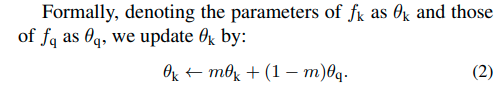
이때, key parameter는 back propagation으로 update되지 않고, query encoder만 update된다.
위 식에 의해서 key encoder는 query encoder에 비해서 더 천천히 update되는 효과를 가져다 준다.
이러한 방법을 통해 queue에 있는 key들은 different encoder에 의해서 encoding이 되지만,
2개의 encoder에 의해서 encoding된 결과의 차이는 줄어들게 된다.
실험결과에 따르면 momentum value가 클수록 더 좋은 결과가 나왔다. (m=0.999 > m=0.9)
Shuffling BN
f_q , f_k 모델 둘다 batch normalization을 사용하는데, 실험결과 BN이 good representation을 학습하는데 오히려 방해가 됨을 확인하였다. BN 과정에서 생기는 batch 내부 안의 정보 공유가 학습을 방해하는 것으로 추측하고 있다.
그리고 저자들은 이 문제를 shuffling BN으로 해결하고 있다.
key encoder f_k 에 대해서 mini-batch의 sample order를 shuffle한다. 그리고 GPU로 전달한다.
그리고 encoding이 끝나면 shuffle 된 것을 다시 되돌린다.
그리고 query encoder f_q의 sample order는 변경하지 않는다.
즉, query와 positive key가 다른 batch상에서 나와야 하며, 같은 batch에 있는 경우 batch normalization 계산과정에서
정보를 공유하는 부분 때문에 더 좋은 representation 학습에 방해가 된다.
Paper
Learning Imbalanced Datasets with Label-Distribution-Aware Margin Loss
Deep learning algorithms can fare poorly when the training dataset suffers from heavy class-imbalance but the testing criterion requires good generalization on less frequent classes. We design two novel methods to improve performance in such scenarios. Fir
arxiv.org
Code
kaidic/LDAM-DRW
[NeurIPS 2019] Learning Imbalanced Datasets with Label-Distribution-Aware Margin Loss - kaidic/LDAM-DRW
github.com
Introduction
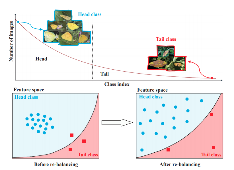
Imbalanced data 문제는 보통 re-weighting, re-sampling 접근 방법을 많이 사용한다. 이는 train data distribution과 test data distribution을 동일하게 만듬으로써, 문제를 접근한다. 하지만 결국 minority class의 sample의 부족은 overfitting을 발생시킨다는 것은 큰 어려움이다.
그래서 저자는 majority class에 비해 minority class에 강한 regularizing 기법을 적용함으로써, minority class에 대한 정확도를 향상시키는 방법을 제안한다.
이는 기존의 weight matrix에만 regularization 방법을 적용한 것과 달리, label에도 함께 regularization 방법을 적용한다.
결론적으로 본 논문에서는 label-distribution-aware loss function을 적용함으로써, model의 margin을 minority class에 대해 좀 더 크게 되도록 최적화한다.
Main approach
1) Problem setup and notations
2) Fine-grained generalization error bounds.
일반적인 generalization error bound는 다음과 같다. (training , test data distribution이 동일한 경우)
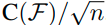
이는 모델의 복잡도가 증가할수록 overfitiing이 잘되기 때문에, 복잡도에 비례하게 되고, training data 수가 많을수록
실제 data의 분포에 맞게 학습이 가능하기 때문에 error bound가 작아지게 된다.
그리고 training, test 모두 동일하게 imbalanced distribution인 경우, error bound는 다음과 같이 형성된다.
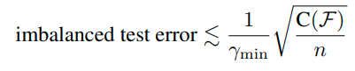
위의 식의 의미는 class간의 margin중에서도 최소값인 r_min이 크다는 것은 class 간의 boundary가 잘 형성되어있다는 의미이고, error의 최대값이 작아진다는 의미이다.
그러나 위 식에서는 label distribution에 대한 정보는 나타나 있지 않다.(oblivious)
그래서 다음과 같이 fine-grained하여 loss function을 다시 구성한다.
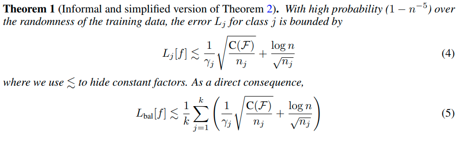
3) Class-distribution-aware margin trade-off
위의 margin 식을 살펴보면 class에 대한 sample의 수가 많을수록 error bound가 작아지는 것을 확인할 수 있다.
즉, minority class에 대한 error bound를 줄이려면 margin값을 크게 해야한다는 사실을 알 수 있다.
그러나 minority class에 대해 margin을 너무 크게 하면, majority class에 margin이 작아지는 단점이 있다.
그렇다면 optimal한 margin은 어떻게 구할 수 있을까?
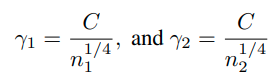
class가 2개인 binary classfication 문제인 경우 balancd generalization error bound를 다음과 같이 나타낼 수 있다.
( 5번식 참고)
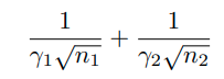
이때, r_1과 r_2는 복잡한 weight matrices이기 때문에 optimal margin을 구하기 어렵다.
하지만 이러한 방식으로 접근이 가능하다. 만약 margin r_1, r_2가 현재 optimal이라면,
shifted bias를 현재 margin에 적용했을때, 아래와 같이 error bound가 더 커져야 한다.
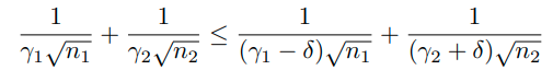
위 식은 다음과 같은 의미를 내포한다.
4) Fast rate vs slow rate, and the implication on the choice of margins.
generalization error bound에는 Fast rate와 slow rate라는 용어가 있다.

의 scale에 따라 bound가 변화하는 경우, 'slow rate'라고 부른다.

위와 같이 변화하는 경우 'fast rate'라고 부른다.
딥뉴럴넷이 충분히 큰 경우 위와 같이 fast rate로 바뀔 수 있다.
Label-Distribution-Aware Margin Loss
위의 binary classificaiton의 경우를 고려하여 저자는 multiple case에 대해서 다음과 같이 가정한다.
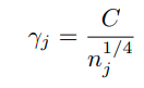
그리고 soft margin loss function을 위와 같은 margin을 가지도록 디자인한다. (optimal margin이므로)
(x,y)를 training example이라고 하고, f를 모델이라고 하자. 이때,
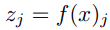
를 model의 j class에 대한 output이라고 정의한다.
이때 hinge loss를 이용해서
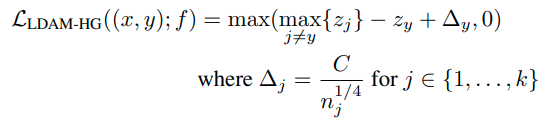
위와 같이 loss function을 구성가능하다.
위 식의 의미는 다음과 같다. label y에 대한 logit과 다른 클래스 logit의 max값의 차이가 최소 △는 되어야 한다.
그러나 hinge loss가 smooth 하지 않은 점은 optimization 과정에서 문제점을 만들어내고, 다음과 같이 cross-entropy loss에 margin을 부여해서 smooth한 hinge loss를 만들어 낼 수 있다.
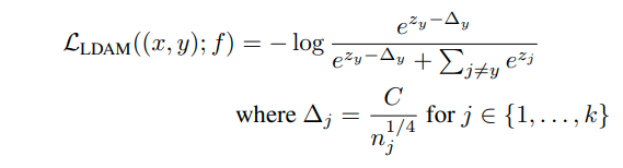
label y에 대한 logit이 margin보다 커야 loss값을 줄일 수 있음
Deferred Re-balancing Optimization Schedule
re-weighting 방법과 re-sampling 방법은 imblanced dataset을 다루는 주요한 방법이다.
(둘다 uniform한 test distribution에 가깝게 만드는 방법이기 때문)
그러나 re-sampling 방법의 경우 model이 deep neural network인 경우 heavy overfitting이 나타난다고 알려져 있다.
그리고 re-weighting의 경우 optimazation이 불안정하다는 단점이 있다. (특히 extremely imbalanced인 경우)
그래서 이전 연구에서 이러한 optimization 문제를 다루기 위해 복잡한 learninig rate schedule을 적용한 바가 있다.
저자들은 re-weighting , re-sampling 방법 모두다 learning rate를 적절히 annealing 하지 않는 경우,
ERM보다 오히려 성능이 떨어지는 것을 발견하였다. (all training example에 대해 똑같은 weight를 주는 방법)
annealing을 하기 전에 re-sampling 및 re-weighting 방법으로 생성된 feature의 경우 오히려 안좋은 것으로 확인되었다.
그래서 다음과 같은 defered re-balancing training procedure를 만들었다.
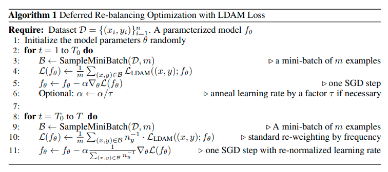
먼저 LDAM loss를 vanila ERM (no weighting) 방법을 사용하여 training 시킨다. 그리고 이후에 smaller learinig rate를 이용해 re-weight LDAM loss를 적용한다. 실험 결과적으로 training의 first stage(no weighting) 는 second stage(weighting)의 좋은 초기화 방법이 된다.
Experiments
1) Baselines
(1) ERM loss : 모든 example에 대해서 똑같은 weight를 적용한 방법, standard cross-entropy loss를 사용한다.
(2) Re-Weighting(RW) : class의 sample size에 inverse하게 weighting한다.
(3) Re-Sampling(RS) : 각 example을 sampling할때, class sample size에 inverse하게 sampling
(4) CB : Class-balanced loss based on effective number of samples 논문 참고
(5) Focal Loss : Focal loss for dense object detection. 논문 참고
(6) SGD schedule : SGD를 learning rate dacay method 방법을 사용한 것.
2) Our proposed algorithm and variants.
(1) DRW and DRS : 먼저 Algorithm 1에 적힌 것 처럼 standard ERM optimization을 적용하고 그 다음 second stage때 re-weighting 및 re-sampling 방법을 적용하는 것을 말한다.
(2) LDAM : 본 논문에서 제안된 Loss function을 적용한 것.
3) Experimental results on CIFAR
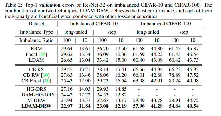
HG-DRS 는 Hinge Loss+DRS
LDAM-HG-DRS는 Hinge Loss에 LDAM margin을 준 것,
M-DRW는 cross-enropy에 uniform margin을 줘서 사용한 것을 말한다.
Hinge Loss의 경우 100 class에서 optimization 이슈가 있어서 10개 클래스에서만 실험하였다.
Conclusion
1) LDAM loss를 통해 최적화 된 class 별 margn을 찾음 (binary를 통한 추론값을 multi class에 적용
2) 학습 초반 부터 re-weighting 및 re-sampling 기법을 적용하면 feature의 학습이 저해되는 부작용이 있는데,
처음에는 standard training 방법을 사용하고 이후에 re-weighting 및 re-samping을 적용하는 deferring 방법을 사용함.
| Fov (Field of View) (0) | 2021.02.22 |
|---|---|
| End-to-end learning (0) | 2021.01.11 |
| Bayes optimal classifier (0) | 2021.01.04 |
| Gaussian mixture model (0) | 2021.01.01 |
| Focal Loss (0) | 2020.12.30 |
Paper
Rethinking the Value of Labels for Improving Class-Imbalanced Learning
Real-world data often exhibits long-tailed distributions with heavy class imbalance, posing great challenges for deep recognition models. We identify a persisting dilemma on the value of labels in the context of imbalanced learning: on the one hand, superv
arxiv.org
Code
github.com/YyzHarry/imbalanced-semi-self
YyzHarry/imbalanced-semi-self
[NeurIPS 2020] Semi-Supervision (Unlabeled Data) & Self-Supervision Improve Class-Imbalanced / Long-Tailed Learning - YyzHarry/imbalanced-semi-self
github.com
Introduction
일반적인 supervised learning에서는 data의 label은 무조건 도움이 된다.
unsupervised learning과 비교해보면 그것을 알 것이다.
그러나 imbalanced learning에서는 상황이 달라진다.
majority class에 의해 decision boudary가 강하게 형성되게 되고,
아래와 같이 decision boudary가 형성되는 경향성을 보이게 된다.
그래서 다음과 같은 의문을 제기 한다.

그래서 본 논문에서는 imblanced learning에서의 label의 positive한 면과 negative한 면을 살펴보고 이를 semi-supervised learning과 self-supervised learning 방식으로 이용하여 sota를 달성했다.
먼저 positive view는 imbalanced label이 유용하다는 것이다. 그래서 extra unlabeled data를 추가적으로 사용하여 psedo-labeling data를 형성하고 이를 통해 semi-supervised 방식으로 추가적인 학습을 진행하면, imblanced data 학습을 통한 성능이 향상된다는 것을 증명하고 있다.
그리고 negative view는 imbalanced label이 항상 유용하지는 않다는 것이다. imbalanced label만을 이용해 학습할 경우 acc의 최대치의 bound가 정해지게 된다. 그러나 label을 따로 지정하지 않는 self-supervised 방식을 적용하면 imbalanced label만을 이용해 학습할 경우 제한되는 acc의 한계를 넘을 수 있다는 것이다. 본 논문에서는 이를 수식 및 실험적으로 증명하고 있다.
Imbalanced Learning with Unlabeled Data
먼저 Unlabel Data를 추가적으로 학습에 사용할 때, 어떠한 효과가 있는지 알아보기 위해 이론적으로 살펴본다.
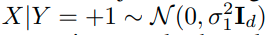
먼저 binary classification 문제를 고려한다. data는 2개의 Gausssian의 mixture P_xy 모델을 사용한다.
label Y는 positive value (+1) , negative value (-1) 2가지를 같은 확률 (0.5)의 확률로 가지게 된다.
그래서 Y=+1 일때, data X의 label이 +1 인 경우는 다음과 같이 normal distribution을 따른다. ( label 1에 대한 u_1 gaussian)

Y= -1 일때, data X의 label이 -1 인 경우는 다음과 같이 normal distribution을 따른다. ( label 2에 대한 u_2 gaussian)
이 경우 optimal bayes's classifier는
가 된다.
이 경우,

가 된다.
이러한 상황에서 base classifier f_b를 정의해보자. (which is trained on imbalanced training data)
그리고 extra unlabeled data

가 주어졌다고 생각해보자.
base classifer f_B를 이용해 unlabeled data에 대해서 psuedo-label을 형성한다.
결과적으로 psuedo-label이 +1인 unlabeled-data set을

psuedo-label이 -1인 unlabeled -dataset을

로 표시한다.
이때, psuedo-label이 +1로 분류된 data가 실제로 label이 +1인 경우 indicator를 사용해 '1'로 표시해준다.

그래서,

이때
가 되고, 의미는 f_B가 Positive class에 대하여 p의 acc를 가진다는 의미이다.
유사하게


가 되고, 의미는 f_B가 Negative class에 대하여 q의 acc를 가진다는 의미이다.
결과적으로
로 정의가능하다.
이러한 상황에서, extra unlabeled data를 이용해,
를 배우는 것이 목표이다.
저 parameter를 측정하는 방법은 아래와 같이 측정이 가능하다.

이때 다음과 같은 결과를 얻을 수 있다.
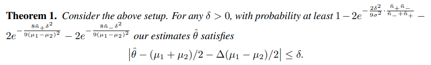
이 결과는 다음과 같이 해석할 수 있다.
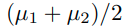
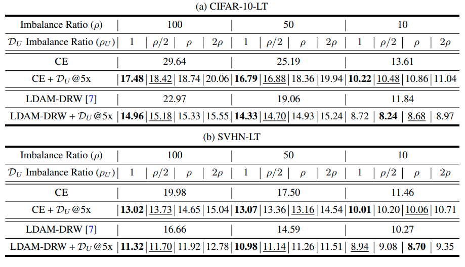
1) Training data imabalance를 estimation의 정확도에 영향을 준다.
위 수식을 보면 △ 가 estimation에 영향을 주는 것을 확인 할 수 있다. 즉, imbalance 정도가 estimation에 영향을 준다.
2) unlabeled data의 imbalanced 정도는 good estimation을 얻을 확률에 영향을 준다.
이때, unlabeled data가 balanced인 경우 good estimation을 확률이 증가한다.
그러나 unlabeled data가 balanced하지 않더라도 어찌되었든 imbalanced data를 추론하는 것에는 도움이 된다.
Semi-Supervised Imbalanced Learning Framework
이러한 가설을 기반으로 본 논문에서는 "Semi-Supervised Imbalanced Learning Framework"를 제안한다.
먼저 original imbalanced dataset 으로 부터 학습시킨 intermediate classifier 'f' 를 얻는다.
그리고 이 'f'를 이용하여 unlabeled data D_u로 부터 pseudo-label y를 생성한다.
이를 이용하여 최종 모델 f는 다음과 같은 Loss식을 이용해 얻는다.
여기서 w는 unlabels weight이다.
이 방식은 다른 어떠한 SSL 방식에도 적용이 가능하기 때문에 더욱 실용적이다.
Experimental Setup
실험은 2가지 dataset에서 진행되었다.
CIFAR-10, SVHN
CIFAR-10의 경우 CIFAR-10에 유사한 Tiny-imagenet class data를 unlabel data로 사용한다.
SVHN의 경우 extra SVHN dataset을 unlabeled dataset으로 사용한다.
Why good?
이건 SSL을 좀 더 이해해야 될듯
Experiment results
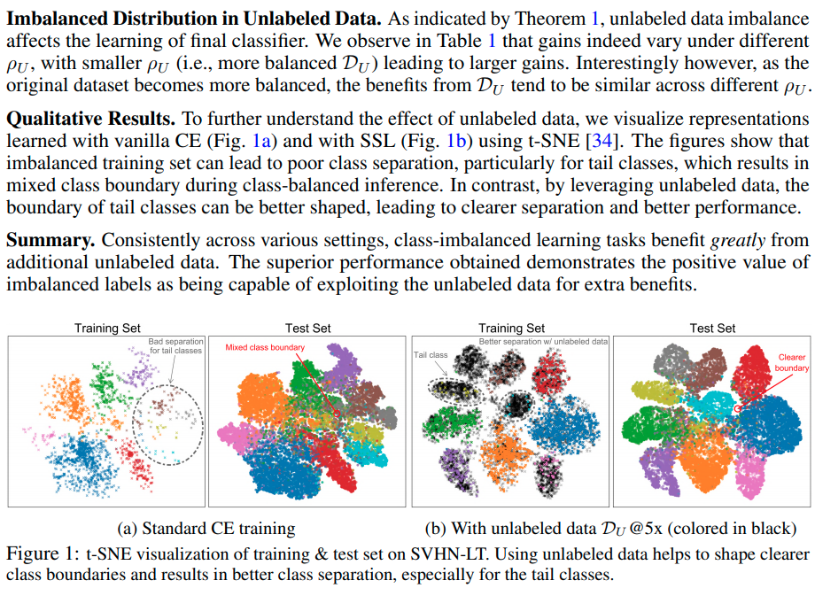
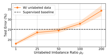
A Closer Look at Unlabeled Data under Class Imbalance
이러한 SSL 방식을 통해 unlabel data를 이용하는 방법은 unlabel data와 original data의 distribution match가 잘맞는 것이 중요하다.
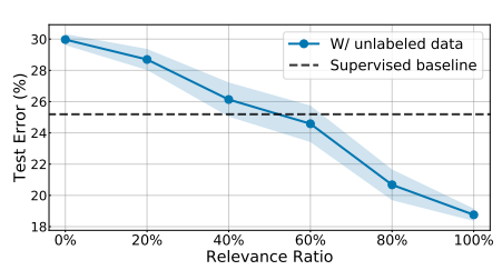
- Data relevance가 낮으면 성능에 저해가 된다. 기준은 Relevance ratio 60% 이다.
Imbalanced Learning from Self-Supervision
Imbalaced data의 label은 어찌되었든 bias를 가지고 있기 때문에 classification 성능에 악영향을 끼치게 된다.
따라서 본 논문에서는 label을 따로 지정하지 않는 self-supervision 방식을 도입하여 성능 향상이 가능함을 보여준다.
먼저 이론적으로 self supervision이 도움이 되는 것을 증명하기 위해 다음과 같은 상황을 가정한다.
d-dimension binary classification, data distribution P_xy mixture Gaussian을 가정한다.
이때, Y=+1은 prob p_+ 를 가지고, Y=-1은 prob p_-를 가진다. (p_- = 1-p_+) 그리고 p_-는 0.5보다 큰 것을 가정한다.
(major class를 negative로 정의하기 때문임)
Y= +1, X는 d-dimensional isotropic Gaussian이라고 정의할 경우,
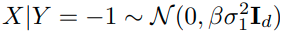

이유는 negative sample이 더 큰 variance를 갖기 때문이다.
(majority class는 sample수가 많고 그 이유 때문에 큰 variance를 갖는다.)
이 상황에서 self-supervision을 적용하기 전과 적용한 후를 비교하기 위해 linear classifier에 self-supervision을 적용하기 전과 후를 비교할 예정이다.
linear classifier를
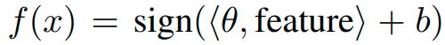
여기서 'feature'는 standard training을 통해 배우는 feature이다.
self-supervised learning을 통해 배우는 feature는 다음과 같이 표현한다.
이때 다음과 같은 결과를 도출할 수 있다.

Theorem 2는 standard training으로는 3/4이상의 acc를 가지지 못한다는 것을 이야기 한다. (B가 3일때)
그러나 self-supervision을 통해 Z를 추출하면 더 높은 정확도를 얻을 수 있다.

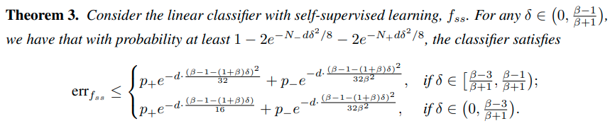
위의 내용은 다음과 같은 내용을 의미한다.
처음에 imbalanced dataset의 label을 제거한 후, self-supervised 방법을 통해 f_ss 를 만든 후 imblanced learning을 하는 경우 더 좋은 성능을 보이게 된다.
Self-Supervised Imbalanced Learning Framework
SSP 를 적용하는 방식은 다음과 같다. 먼저 self-supervision 방식을 통해 f를 학습시킨 후, standard training 방식을 적용하여 final model을 만든다. 이러한 방식은 어떠한 imbalanced learning method에 적용이 가능하기 때문에 장점이 있다.
Experimental Setup
RotNet이랑 MoCo를 사용함.
학습은 pretrain, standard train 모두 같은 epoch 적용 (CIFAR-LT 200 epoch , ImageNet-LT 90 epoch)
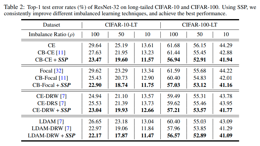
results
A Gentle Introduction to the Bayes Optimal Classifier
The Bayes Optimal Classifier is a probabilistic model that makes the most probable prediction for a new example. It is described using the Bayes Theorem that provides a principled way for calculating a conditional probability. It is also closely related to
machinelearningmastery.com
Bayes optimal classifier는 새로운 example에 대해서 가장 확률적으로 그럴 듯환 prediction을 결과를 도출하는 확률 모델이다.
이는 Bayes Theorem을 기반으로 하며, MAP로 가장 확률적으로 그럴듯한 결론을 도출한다.
Bayes Optimal Classifier는 실제로 계산하기에는 너무나 복잡하다. 그러나 Gibbs algorithm 및 Naive Bayes로 approximation하여 결과를 도출한다.
Meachine learning에서 traing data를 가장 잘 설명하는 모델을 찾는 것이 목적이다.
이때 기반으로 사용되는 확률 이론이 크게 2가지가 있다.
이 이론을 이용하여 다음과 같은 질문에 대답할 수 있다.
What is the most probable hypothesis given the training data?
이때, Bayesian method로 접근 할 경우, 다음과 같이 X(data)가 주어졌을 때,
P(parameter)의 확률을 다음과 같이 표현할 수 있다.
P(theta | X) = P(X | theta) * P(theta)
이러한 테크닉을
“maximum a posteriori estimation,” or MAP estimation for short, and sometimes simply “maximum posterior estimation.”
이라고 보통 부른다.
결론적으로는
maximize P(X | theta) * P(theta)
를 하는 parameter를 찾는 것이 목적이 된다.
Bayes optimal Classifier는 다음과 같은 질문에 해답을 주는 classifier다.
What is the most probable classification of the new instance given the training data?
그리고 다음과 같은 이름으로 불린다.
The Bayes optimal learner, the Bayes classifier, Bayes optimal decision boundary, or the Bayes optimal discriminant function.
일반적으로 가장 확률적으로 그럴듯한 new instance의 classification 결과는 모든 hypotheses의 prediction을 그들의 posterior porbabilities의 weighted sum으로 결정된다.
이를 수식으로 표현하면 다음과 같다.
P(vj | D) = sum {h in H} P(vj | hi) * P(hi | D)
vj is a new instance to be classified,
H is the set of hypotheses for classifying the instance,
hi is a given hypothesis,
P(vj | hi) is the posterior probability for vi given hypothesis hi,
P(hi | D) is the posterior probability of the hypothesis hi given the data D.
이때, 결과는 다음과 같이 결정한다.
max sum {h in H} P(vj | hi) * P(hi | D)
이 수식을 통해 example을 classify 하는 모델을 Bayes optimal classifier라고 하며,같은 hypothesis space와 같은 prior knowledge를 사용하는 경우, 다른 어떤 classification method도 이 성능을 넘지 못한다.
이 말 뜻은 같은 data, 같은 hypotheses, 같은 prior probabilities를 이용하는 경우 어떤 알고리즘도 이 방법의 성능을 넘지 못한다는 것이고, 그래서 “optimal classifier.” 라고 부른다.
비록 이 classifier는 optimal한 prediction을 하지만, 완벽한 classifier는 아니다. training data의 uncertatiny 및 problem domain과 hypothesis을 모든 경우에 고려할 수는 없기 때문이다.
그래서 이러한 optimal classifier도 error를 가지며, 이를 Bayes error라고 한다.
즉, Bayes Optimal Classifier는 lowest possible test error rate를 가지며, 이를 bayes error rate라고 부른다.
이는 더이상 줄일 수 없는(irreducible) error와 같다.
Bayes Error: The minimum possible error that can be made when making predictions.
| End-to-end learning (0) | 2021.01.11 |
|---|---|
| Sampling with replacement (0) | 2021.01.07 |
| Gaussian mixture model (0) | 2021.01.01 |
| Focal Loss (0) | 2020.12.30 |
| imagenet pretrained model에서 imagenet data 분포로 normalize하는 이유 (0) | 2020.12.30 |
https://towardsdatascience.com/gaussian-mixture-models-explained-6986aaf5a95
Gaussian Mixture Models Explained
In the world of Machine Learning, we can distinguish two main areas: Supervised and unsupervised learning. The main difference between…
towardsdatascience.com
| Sampling with replacement (0) | 2021.01.07 |
|---|---|
| Bayes optimal classifier (0) | 2021.01.04 |
| Focal Loss (0) | 2020.12.30 |
| imagenet pretrained model에서 imagenet data 분포로 normalize하는 이유 (0) | 2020.12.30 |
| 활성화 함수 nonlinear 이유 (0) | 2020.12.14 |
Imblanced Sampling distribution: Pareto dustribution a=6

many class : over 100 sample
medium class :20~100 sample
few class : under 100 sample
Class-aware sampling
| Open Set Learning with Counterfactual Images : ECCV 2018 (0) | 2021.07.07 |
|---|---|
| Generative OpenMax for Multi-Class Open Set Classification : BMVC 2017 (0) | 2021.06.29 |
| Toward Open Set Deep Networks : CVPR 2016 (0) | 2021.06.28 |
| Learning Placeholders for Open-Set Recognition: CVPR 2021 Oral (0) | 2021.05.21 |
| Learning Open Set Network with Discriminative Reciprocal Points : ECCV 2020 (0) | 2021.01.19 |